How to recover lost rides on Strava

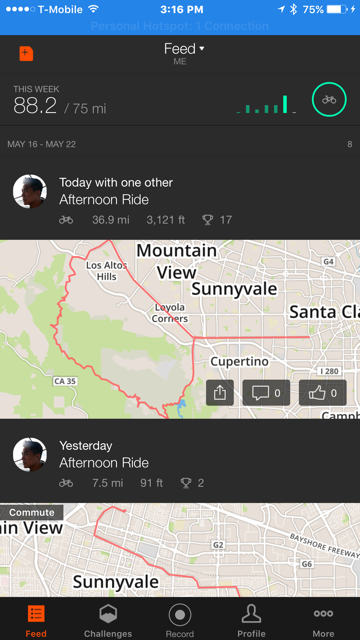
I recently started biking, and the fact that I’ve kept at it is due in no small part to Strava.  I really like tracking my progress, seeing how I compare to others and myself.  I’ll admit on more than one occasion, I’ve chosen to ride just to see those weekly numbers tick up.

My obsession with stats can obviously only be sated with more stats.  After putting in the time on long rides, I pore over each segment seeing how my performance stacked up from week to week.  Today, I went on a long ride (~37 miles) going up Montebello road and then down Page Mill.   I huffed and puffed, facing cold rain atop Black Mountain, a sore elbow and unhealthy wobbles descending on the dirt road that almost ended with me eating shit. Yet I was happy to do it all so I could see my stats.

strava2
random strava logo

Then the terrible occurred – when I went to upload the file, nothing appeared in my feed. I waited … then waited some more … and then some more.  It still wouldn’t appear!  I tried recording another activity just to make sure I was able to upload files and it recorded just fine.  Mortified, I thought my three hour suffer-fest would end with nothing to show for it (because in reality, what’s the point of riding without obsessing over times?).

Disclaimer: To be fair, I’m not sure I waited the entire time for my file to upload (it was pretty big, around 2.9 MB, and speaking of which Strava, I highly suggest you compress the files before upload, it would make them so much faster to upload), but still I thought that it was just taking the Strava servers some time to process.

However, it turns out that after a little digging in, I was able to recover the file and successfully upload it to Strava’s servers.  Here’s the process to do so, so your precious activity doesn’t go uncollected.

First some context:

I have an iPhone 6 plus, running iOS 9.3.2 and Strava v.4.16.0 (4015).

Steps:

1. First, make sure the file is still on your mobile device.  On the iPhone, you can connect your phone, open up iTunes, and navigate to Apps/Strava where you can see all of your activities.  Here’s what it looks like: 

Note: If you don’t have this file anymore, unfortunately I think you’re hosed.  You can always try to contact Strava to see if your file is on their server somewhere.

Screen Shot 2016-05-21 at 3.26.59 PM
iTunes strava app data view

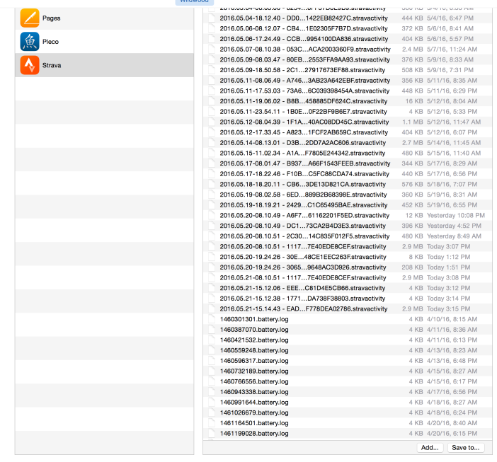
2. Next, locate the file that failed to upload to Strava.  This may take a little bit of guess and check, however if it’s your latest activity, you’ll see it sorted by timestamp so it should be at the end:

Screen Shot 2016-05-21 at 3.27.51 PM

3. The next part is a little tricky.  You can save the file to your local machine by right-clicking “Save to…”.  And then you can open the file in a text editor.  I used sublime text (hey I’m a dev).  The file will be huge and looks something like this:

Sample file:

strt: t:485449851.286994
lvseg: t:485537646.134324 on:1
wp: lat:37.337964; long:-121.979434; hacc:5.000000; vacc:3.000000; alt:38.173744; speed:3.720000; course:268.593750; t:1463844846.142122; dt:1463844846.142122; dist:7.644818
wp: lat:37.337964; long:-121.979434; hacc:5.000000; vacc:3.000000; alt:38.173744; speed:3.720000; course:268.593750; t:1463844846.142135; dt:1463844846.142135; dist:7.644818
relv: v:0.977640; t:1463844846.825438;

Side note on understanding the file.  I don’t work for Strava, so I’m just spitballing here, but the file is obviously appended to as your activity takes place.  Here are some guesses as to what each datapoint means:

strt: looks like start

  • t: unsure.  At first I thought timestamp, but the value is way too low (resolved to somewhere in 1985).  So still a mystery.

lvseg: looks like live segment

  • given that strava just added this, I’m going to guess that this means you’re doing a live segment and on: 1 means it’s recording

wp: looks like these are the main data points

  • lat: latitude
  • long: longitude
  • hacc/vacc: horizontal/vertical acceleration
  • alt: altitude
  • speed: self explanatory
  • course: unsure
  • t: start timestamp
  • dt: end timestamp
  • dist: distance (in kilometers, I think)

relv: relative velocity (maybe)

So essentially, by looking at the latitude and longitude and timestamp, you can figure out where you were at what time.  It’s a little bit tedious to do so (if you’re trying to upload an old file), however you can avoid this if it’s your most recent activity.

4. My Strava refused to upload this file (also, it had a timestamp in the past), so I’m guessing that somewhere on your mobile device strava marks certain events that you decide not to upload and skips over them when the app boots up.  

To work around this limitation, I simply recorded a new activity and brought myself to the screen before the “save” screen.  

Don’t hit “save” yet.

You can see in iTunes that a new file was generated with the correct timestamp.  I next clicked “Save to …” to copy this to my local machine, where I brought it up in sublime again.  Note the UUID (DF5…857A831ECFD) looking thing so you can locate the file after you copy it locally.

Screen Shot 2016-05-21 at 3.36.17 PM

The file looks like this (note how small it is since we only recorded about 9seconds worth; also maybe interesting, Strava filling up your phone maybe @ 0.5 – 1KB/second means that each hour of activity is very roughly few MB, probably depends on the # of breaks you take):

lvseg: t:485562945.972006 on:1
strt: t:485562945.983277
wp: lat:37.338599; long:-121.978195; hacc:10.000000; vacc:32.000000; alt:54.916534; speed:0.620000; course:-1.000000; t:1463870147.006819; dt:1463870147.006819; dist:0.000000
wp: lat:37.338570; long:-121.978124; hacc:10.000000; vacc:12.000000; alt:42.931915; speed:0.000000; course:-1.000000; t:1463870148.002843; dt:1463870148.002843; dist:0.000000
relv: v:0.000000; t:1463870148.671240;

Next what I did is copy the contents of the original file into this file, essentially deleting everything in this file after the “strt: t:485562945.983277”.  Not sure if this is strictly necessary, but at any rate, it probably doesn’t hurt.

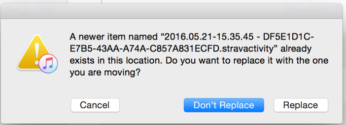
5. Finally, the last step is to copy the modified file (with the same filename) back to iTunes.  iTunes will prompt you for whether you want to overwrite the file.  Hit “Replace”.

Screen Shot 2016-05-21 at 3.40.30 PM 

Now you’ll see that the file changes size on your iPhone.

Screen Shot 2016-05-21 at 3.41.34 PM

8. Now you can hit “save” on your Strava app.  If you did everything right, you’ll see that the activity gets uploaded and parsed by Strava’s servers.  If it’s a large file, it may take some time.

That’s it!  Your precious stats are back.

Note to Strava developers: you can probably encrypt these files rather than store them in plaintext.  I’m not saying I would ever mess with the GPS coordinates or timestamps to hack my way to King of the Mountain status or anything, but others might. 😉

IMG_7502
Hooray! I have a reason to ride again!


Search Part VIII: Online Compressed Prefix Tries

In the previous blog post, I discussed autocomplete with wild cards.  That implementation was based on simple prefix tries, where each character in each word maintained a separate node.  Insertion, removal, and traversal of the simplistic prefix trie is easy; We simply traversed along the path per character in the word being looked up.  If we fell off the path, we knew that the word wasn’t in the dictionary; if we didn’t, we could determine whether the word was in the dictionary by checking the whether terminal = true, and further traverse to generate a set of all suffixes with that prefix.

In this blog post, I take that implementation one step further and implement insert, remove and traverse for a compressed prefix trie.  What are the advantages of a compressed prefix trie?  Essentially, the implementation is superior in every way except complexity compared with a simple prefix trie.

See the implementation here (and feel free to play with it): Search Part VIII: Compressed/Optimized Prefix Tries

Advantages of Compression

As stated above, the advantages of compression are numerous.  Here are a few below:

  • Significantly reduce memory footprint.  In my personal tests, I end up using around 66% less memory
  • Faster traversal and results generation.  Since compressed tries can simply traverse along the value kept in each node vs having to traverse down the trie, lookup is significantly faster as well (up to 66% faster)
  • Faster construction of the trie.  The same advantages above apply.

A compressed trie

What is a Compressed Trie?

A compressed trie builds upon a normal trie by eliminating redundant edges in the trie.  In my implementation, I compress down each branch (representing each suffix).  I could go even one step farther and use pointers to existing substrings in the trie.  Using this approach, I’ve heard of compressibility/memory savings using only 16% compared with a full-blown trie.

The best way to explain how a compressed trie works is to compare the non compressed with the compressed versions (* represents terminal nodes):

2.1.7 :007 > a.prefix_trie.print

  a
    p
      p
        l
          e*
  b
    a
      n
        a
          n
            a*
              s*
  m
    a
      n
        g
          o*
            e
              s*
            s
              t
                e
                  i
                    n*
  g
    r
      a
        p
          e*
  p
    i
      n
        e
          a
            p
              p
                l
                  e*

Total size: 39 nodes

Compare this with a compressed trie:

  apple*
  banana*
    s*
  mango*
    es*
    stein*
  grape*
  pineapple*
 => nil

Total size: 9 nodes

Thus, right off the bat, you can see that the size has shrunk by 30 nodes, or ~ 75%.  Of course, real memory savings is a little more vague, since each flattened node is now larger by holding a larger value.

What changed from the uncompressed to the compressed trie?  Essentially, you can see that each branch of the trie that only had one child could be compressed into the same node.  For example, pineapple is the only word that starts with p in the dictionary, thus each edge could be compressed down to one word.

In practice, a flattening algorithm would look like this:

        var node = this;
        while (node.num_children() === 1 && !node.terminal) {
            //set children to child 
            var child = node.children[Object.keys(node.children)[0]];
            var grandchildren = child.children;
            node.children = grandchildren;
            node.c += child.c;
            node.terminal = child.terminal;
            _.each(grandchildren, function(gc) {
                gc.parent = node;
            });
            if (child.terminal) { break; }
        }

This algorithm simply traverses up the chain, squashing any redundant edges along the way. Next, if we apply this across all leaf nodes, we can optimize the entire trie.

    this.optimize = function() {
        var self = this;
        var queue = [];
        Object.keys(self.children).forEach(function(k) {
            queue.push(self.children[k]);
        });
        while (queue.length > 0) {
            var node = queue[0];
            node.flatten();
            Object.keys(node.children).forEach(function(k) {
                queue.push(node.children[k]);
            }); 
            queue = queue.splice(1);  
        };
    };

The next step is to rewrite the traversal algorithm, because we can’t naively use each character in the word we are trying to look up to traverse each node.  We need a way to tell if the current node we are at is a flattened node or not.  If so, traverse into the word as far as possible and return where we all off, or if we’re done traversing, return the node.  In practice, it’s a little more complex than that, and there are lots of tricky edge cases in the implementation.  However, I’ve done the hard work for you:

/* traverses tree based on text */
    this.traverse = function(textIn) {
        var node = this;
        var path = '';
        var j = 1;
        var dist = j;
        var chars = textIn.split('').map(function(c) { return c.toLowerCase(); })
        
        /* traversal of compressed trie */
        for (var i = 0; i < chars.length; i++) {
            c = chars[i];
            if (node.flattened()) { // flattened
                if (node.c[j] === c) {                
                    path += c;
                    j++;
                    dist = j;
                    continue;
                } else if (j < node.c.length) { //terminated early
                    return [path, undefined, node, j];
                }
                j = 1;
                
            }
            if (node.children[c]) {
                path += c;
                node = node.children[c];
                //already added path above
            } else {
                return [path, undefined, node, dist];
            }
        }
        var prefix = path;
        if (node.flattened()) { 
            prefix = path.substr(0, path.length - j); 
        }
        return [prefix, node, node, dist];
    };

Essentially, this traversal algorithm does the following. It navigates through the trie for each character in the word being looked up. We go as far as possible until we have to fall off the trie, or have exhausted the characters in the word. After we finish this process, we return a 4-tuple (an array here) below:

# 1) the path taken thus far
# 2) the node traversed into
# 3) if no node traversed into, the last node seen
# 4) the distance into the last node seen

With this information, we have everything we need to either remove the node, insert new nodes from this point, determine whether the word exists in the trie, or continue traversing to complete the suffix set.

Online vs Offline Construction

By following this approach, we’ve derived the compressed trie data structure.  However, we arrived at an offline algorithm for actual construction; that is, we need the entire corpus of words in the dictionary to construct the trie.  Then, once we have constructed the entire trie, we need to traverse the entire trie again and flatten every branch, essentially doubling the amount of effort for trie construction.  On very large datasets, this can be costly.  This is known as an offline algorithm, or one that requires the whole dataset in order to construct the output.  Contrast this to an online algorithm, which can produce the desired output incrementally.  The implementation of the online algorithm for compressed prefix trie construction is very tricky.  There are lots of edge cases, maintaining state so we know how far into the trie we’ve gone, and taking slices of prefixes so we can continue splitting nodes and swapping children.  I’ll just describe it here, but you can see the implementation for the gory details.

Online Prefix Trie Construction Algorithm

  1. traverse as deep as we can go, using the above traverse method
  2. if we fall off the trie (i.e. traverse to a dead end)
    1. if we’re at a flattened node
      1. traverse as far into the node as possible, then create a new child node with the remainder of the word
      2. create a new child node with the remainder of the value that was in the node and point all existing children to that node
    2. if not
      1. insert a child node with the remainder of the word
  3. if we don’t fall off the trie
    1. if we reach and leaf node and have consumed all characters, simply set the node to terminal
    2. otherwise, determine how far we’ve gone in the current node
      1. create a child node with the remainder of the value of the node and point all existing children to that node
      2. create a child node with the remainder of the word

Benchmarking

Ok so now for some real world results (Based on a ruby implementation, hopefully to be open-sourced soon):

BEFORE:
Dictionary size: 86036.  Running through creation 5 times.
            user     system      total        real
creation: 10.880000   0.290000  11.170000 ( 11.173094)
>avg:   2.176000   0.058000   2.234000 (  2.234619)
Dictionary size: 86036.  Running through prefix traversal 1000 times.
       user     system      total        real
prefix:  3.010000   0.010000   3.020000 (  3.009824)
   0.003010   0.000010   0.003020 (  0.003010)
Dictionary size: 86036.  Running through suffix traversal 10000 times.
       user     system      total        real
suffix: 12.020000   0.030000  12.050000 ( 12.050301)
   0.001202   0.000003   0.001205 (  0.001205)

Dictionary size: 86036.  Running through brute force traversal 1000 times.
       user     system      total        real
brute force: 17.540000   0.230000  17.770000 ( 17.774003)
   0.017540   0.000230   0.017770 (  0.017774)

AFTER:
Dictionary size: 86036.  Running through creation 5 times.
            user     system      total        real
creation:  4.760000   0.080000   4.840000 (  4.879213)
>avg:   0.952000   0.016000   0.968000 (  0.975843)
Dictionary size: 86036.  Running through prefix traversal 1000 times.
       user     system      total        real
prefix:  2.130000   0.010000   2.140000 (  2.149070)
   0.002130   0.000010   0.002140 (  0.002149)
Dictionary size: 86036.  Running through suffix traversal 10000 times.
       user     system      total        real
suffix:  7.660000   0.020000   7.680000 (  7.706711)
   0.000766   0.000002   0.000768 (  0.000771)

You can see that compressed trie construction is > 50% faster, prefix lookups are 33% faster, suffix lookups are ~40% faster.  This is without spending much time optimizing either.

Finally, look at the memory differences:

# using the dictionary.json files

# Uncompressed
2.1.7 :005 > a.prefix_trie.size + a.suffix_trie.size
 => 575978 (# nodes)

# Compressed
2.1.7 :007 > a.prefix_trie.size + a.suffix_trie.size 
 => 229498 (# nodes)

Double this for maintaining the suffix trie as well for suffix matches.

Thus, we can see that our trie is about 60% smaller than the uncompressed trie. Awesome.

The trie in all its splendor:

I also had some fun and implemented a simple print function that lets you see what the finished trie looks like.  I’ve included a sampling here:

* - terminal node
i*
    n*
      d*
        o
          c
            i
              l
                ity*
                e*
              b
                ility*
                le*
            trinat
              ion*
              e*
          xyl*
            ic*
          -*
            e
              nglish*
              uropean*
            do-chinese languages*
            briton*
            aryan*
            chinese*
          l*
            e
              s*
              n
                t*
                  ly*
                cy*
            in*
          rs
            e*
              ment*
              e*
              d*
            a
              tion*
              ble*
          w*
            ment*
          m
            able*
            it
              e*
              able*
            ptable*
          nesian*
          aniline*
          in*
          or*
            s*
          gen*
            ide*
          phenol*
... and so on

Search Series Part VII – Autocomplete with Wild Cards

In the last post, I discussed using prefix tries for fast autocomplete of words within a dictionary.  In this post, I take it one step further and share some insights that we can glean from prefix tries on how to expand the autocomplete functionality by allowing wildcard search.  You can see the sample implementation here:

Search Part VII – Autocomplete with wild cards

If you recall, prefix trie construction required linear time for construction, O(n) time where n is the number of words inserted into the trie.  We read in each word from the dictionary, and inserted each character starting from the root.  From the prefix trie, we were able to traverse the trie for any prefix, then with DFS or BFS collect all substrings stemming from the node to which we had traversed.  In other words, we were able to quickly find all strings with a prefix of m.

What if we flipped our intuition around and wanted to find all words that contained a particular suffix?  E.g. “ing”, “tion”, “lion”?  We can use the same approach for building the prefix trie to build a suffix trie.

Suffix Trie

A suffix trie follows the same structure as a prefix trie, with nodes each containing a value of one character and a set of child nodes each pointing to a subtrie or to null.  Taking the insight from the prefix trie, we can intuitively see that word’s suffix is essentially a prefix if the word is reversed:  Hence:

“abcdefg” -> “g”, “fg”, “efg”, “defg” etc are all suffixes.  If we reverse the word,

“gfedcba”, we can construct the prefix trie out of the map of reversed words.  So in this case, “g” becomes the root, followed by “f”, “e”, “d”, and so on.

Construction of the suffix trie is trivial, once we have the code in place for constructing the prefix trie.  From our dictionary, all that is needed is to generate a dictionary using each word in reverse, then pass it into our trie constructor.

/* Example: $dictionary starts as  
* $scope.dictionary = {
*     'aardvark': '...',
*     'actor':  '...',
*     'adulation': '...'
* }
*/
        $scope.inverseDictionary = Object.keys(response.data).reduce(function(memo, key) {
            memo[key.reverse()] = response.data[key];
            return memo;
        },{});
/* $dictionary becomes:
* {
*    'kravdraa': '...',
*    'rotca': '...',
*    'niotaluda': '...'
* }
*/

    	$scope.root = toTrie(Object.keys($scope.dictionary));
        $scope.reverseRoot = toTrie(Object.keys($scope.inverseDictionary));

Suffix/Prefix Trie Insights

Note that a suffix trie is essentially a subset of a “suffix tree” which contains pointers to every suffix of every word inserted into the data structure.  Compare this to the simpler approach I’ve taken here which just contains each word in the dictionary.

Now when the user types in a query into the searchbox, we can scan our prefix trie to get a set of all words in the dictionary where the query is a prefix, and simultaneously we can also retrieve a set of all words in the dictionary where the query is a suffix as well (our set of results will be reversed, so we need to reverse them again).  This extends our base functionality with allowing users to specify a wildcard (e.g. ‘*’) in the query string which we can use to scan both tries.  I won’t talk about the trie traversal here, which you can see an implementation of in my past post: Search Series Part VI – Autocomplete & Prefix Tries

Example:

Prefix trie traversal - "act*", would yield ["actor", "acting", etc.]
Suffix trie traversal - "*act", would yield ["exact", "enact", etc.]

Finally, by maintaining both a prefix trie and a suffix trie, we can implement basic intermediate wildcard functionality (up to 1 wildcard).  All we need to do is find the set of prefix results and suffix results and intersect the arrays.

As an aside: why doesn’t this approach support multiple wildcards (e.g. int*me*tion, which would yield [“intermediation”, “intermention”, etc.])?  The answer is the implementation of the suffix trie, which only contains the entire word (as opposed to all suffixes).  If we tokenize int*me*tion into [“int”, “me”, “tion”], we see that me will not return any prefix/suffix results that we expect because with our given prefix and suffix trie, we can only identify words that either begin with “me” or end with “me”, not have “me” somewhere in the middle.  To add this functionality, the implementation would need to be expanded to full blow suffix trees.  (Alternatively, we could also use something more powerful like ternary search trees).

Example:

Prefix & Suffix Tree intersection: "inter*tion", yields ["intersection", "interaction", etc]

(i.e. all matching words were inter is a prefix and tion is a suffix)

Here’s a sample implementation:

var wildcard = function(textIn) {
        if (!textIn) { return; }
        var substrs = textIn.split('*');
        var p = textIn[0] === '*' ? 1 : 0;
        var s = textIn[textIn.length-1] === '*' ? 1 : 0;
        var prefixes = substrs.length > 1 ? substrs.slice(p, substrs.length - 1 + s) : substrs;
        var suffixes = substrs.length > 1 ? substrs.slice(1 - p, substrs.length - s) : substrs;
        
        $scope.results = _(prefixes).map(function(prefix) {
            return $scope.autocomplete(prefix, $scope.root);
        }).flatten().value();
        $scope.reverseResults = reverse(_(suffixes).map(function(suffix) {
            return $scope.autocomplete(suffix.reverse(), $scope.reverseRoot);
        }).flatten().value());
        $scope.intersectedResults = _.intersection($scope.results, $scope.reverseResults);
    };
Example wildcard search
Example wildcard search (inter*tion)
example wildcard search
Example wildcard search (am*ing)

Search Series Part VI – Autocomplete & Prefix Tries

I’ve spent a lot of the last posts demonstrating how to perform full-text fuzzy searches, highlighting, and index generation, and talked about some of the pros and cons of ngram indexing.  This post departs from search and focuses on solving a different problem: autocomplete.  As I mentioned in the first post, there is no silver bullet to search relevance. At Twitter, this means trying to tackle relevance from many angles – index generation, manual ranking of documents, query classification, etc.  Another means of getting better relevance is by trying to guide the user’s query to known queries with good sets of results.  In this post, I’ll demonstrate how to generate build out an autocomplete functionality that can be used to get the user to the right query.

See the sample implementation here: http://Search Series Part VI – Autocomplete

Why autocomplete?

This should be pretty obvious to most readers.  You’ve most likely encountered autocomplete in many places.  For example, when you type into Google’s search bar, you’ll get a list of suggested queries.  When you begin typing an address to Google maps, you’re presented with a list of possible matches.  The google-esque type of functionality probably requires a different solution altogether than the solution I’m proposing.  This post, on the other hand, describes one possible implementation of a way to provide some (but not all) autocomplete functionality.  A slightly non-obvious benefit to autocomplete is that adding autocomplete functionality not only serves as a convenience to the end user, but also is a forcing function that helps to drive search relevance.  By guiding the user to a set of searches with a set of high quality search results, one can help guide the user to those results through query modification.

Trie trie again

A trie (pronounced “try”, as in retrieval) is simply a tree-like data structure where each node in the tree can have 0 -> N leaves.  The familiar binary tree, for example, is a trie which imposes the restriction that each node has at most 2 leaves (a left and right leaf). Prefix tries on the other hand are constructed such that each path to the root is a prefix of the path to the node, where each node contains a character and a set of children.  In other words, if we created a prefix trie as such:


c > o > [d > e, k > e]

In this trie, “code” is one potential path, and each path to the root, “cod”, “co” and “c” are all prefixes of “code”.  However, not all of those prefixes are valid words, so the prefix trie must be able to distinguish between good and bad entries.  In my sample application, I use this use this data structure to efficiently store an entire dictionary, with the guarantee that there is only one path per entry (autocomplete result).  To get to the list of results that can match, I traverse the prefix trie as far as I can go with the user’s query, then use various traversal techniques to find all suffixes for a particular prefix.

Here’s a sample implementation for a prefix trie:

var Node = function(c, parent) {
    var self = this;
    this.c = c; // the value of the node
    this.children = {}; // a map representing the children
    this.parent = parent; // a pointer to the parent
    this.terminal = false; // whether there is a word at this node
    
    /* insert a word at this node */
    this.insert = function(word) {
        if (!word || word.length === 0) { return; }
        ch = word[0];
        if (!self.children.hasOwnProperty(ch)) {
            self.children[ch] = new Node(ch, self);
        }
        var n = self.children[ch];
        if (word.length === 1) { self.children[ch].terminal = true; }
        n.insert(word.substring(1));
    };
};
    

A few words about this implementation:

1) Node – Each node in my implementation has one character as the value and a set of children.  Prefix tries can be constructed with a variety of data structures to represent children for each node (e.g. arrays, linked lists, maps).  In my implementation, I opt to use hash maps for space optimality and constant speed lookup.  However, other popular implementations use arrays or sorted linked lists, which enables a fast sorting of a set of words through a preorder depth first search of the prefix trie (described below).
2) terminal: Boolean – For each word inserted, a path is created from the root node to the leaf node. Thus, it can be assumed that any path from the root node to a leaf node without children is a valid entry. However, there are valid entries that are prefixes of other entries, so there must be a way to distinguish between a valid and invalid path. Hence the terminal flag.
3) duplicates are not stored in the prefix trie (ergo, each path represents a unique result).  We could easily store the number of occurrences of each prefix in the trie.

And here are some interesting properties of prefix tries:
1) Prefix tries can be faster than hash maps for word look up – The longest path to look up a word in the trie takes O(m) time, where m is the length of the word. For a hash map, with a bad hashing function, you could take in the worst case scenario O(n) time, where n is the number of entries in the hash map.
2) Suffix detection – any path to a parent node represents a prefix of all paths through the parent node. Thus, it’s possible (and necessary) to construct an array of all suffixes stemming from the prefix and autocompleting a given result.
3) Sorting – as described above, prefix tries can be used to sort a set of words so long as the children keys are sorted. In this implementation I use hash maps, so the keys are not sorted by default (but we could opt for a different data structure).  Once the prefix trie is constructed, one only needs to traverse via DFS.

4) Prefix tries can be space efficient – Since only all unique prefixes need to be stored in the trie, we don’t need to store needless duplicate keys.

Prefix Trie Traversal

As with typical trees, one can opt for different methods of traversal to construct substrings from a parent node. I’ve provided a few different implementations below.

    /* BFS */
    this.traverseBFS = function(array, prefix, limit) {
        var self = this;
        var queue = [];
        queue.push([self, prefix])
        while (queue.length > 0) {
			var entry = queue[0];
            var n = entry[0];
            var p = entry[1];
			if (n.terminal) {
                array.push(p + n.c);
                if (limit > 0 && array.length >= limit) {
                    break;
                }
            } 
            for (var k in n.children) {
                queue.push([n.children[k], p + n.c])
            }
            queue = queue.splice(1);
        }
    };
    
    /* DFS */
    this.traverseDFS = function(array, prefix, limit) {
        var self = this;
        var keys = Object.keys(self.children);
		for (var i = 0; i < keys.length; i++) { if (limit > 0 && array.length >= limit) {
                break;
            }
            self.children[keys[i]].traverseDFS(array, prefix + keys[i], limit);
        }
        if (!self.terminal || (limit > 0 && array.length >= limit)) {
            return;
        }
        array.push(prefix);
    };

BFS (breadth first search) – With breadth-first search, as we traverse to each child node, we invoke the traverse function call for each child nodes’ children. This is equivalent to traversing by visiting all nodes at each depth before traversing each next level node. This returns matching autocomplete results in order of length. One gotcha here: since BFS uses a queue to control the order of the nodes to visit, we need a way to maintain the prefix up to each node. While each node contains a pointer to the parent, so we could conceivably traverse up to the root node, this would require up to M moves (where m is the length of the word) repeated N times (for each result), resulting in O(MN) time to construct the autocomplete list.

Alternatively, I keep track by simply enqueueing a tuple of the [Node, prefix: String] each time, such that we can construct the autocomplete list by traversing to each node once in O(N) time.

Screen Shot 2015-10-17 at 11.57.04 PM

DFS (depth first search) – With depth-first search, we traverse to the deepest node before starting to recurse. As described above, this method is useful for radix sort if the keys are kept in sorted order (they aren’t in my example). As with normal DFS, we can traverse the tree preorder, inorder or postorder. You can see from my example that I traverse as far left as possible until the left node is a leaf node, then I visit that node, then visit each sibling node called with the prefix up to that point.

depth first search

Some thoughts:

  • Without any intelligence (algorithmic or otherwise), autocomplete only has limited utility in cases where the result set is large.  You can see in this instance, where there are about 109k words in the dictionary, that limiting the user to 10 results probably wouldn’t get the user to the desired query.
  • This current implementation doesn’t account for mispellings in the word or any leniency (e.g. leaving characters out, adding extra characters).  However, we can combine elements of the ngram text search discussed in the first 5 parts of this series. Essentially, the first ngram of a word is also a prefix of the word, so we can use the prefix trie to do some quick filtering, then return a set of fuzzy matches.

Search Series Part V – Search Optimizations (multi-word fuzzy match and highlighting)

In the previous search engine series, I demonstrated how to implement a naive fuzzy match using Levenshtein distance.  I call it naive because the distance metric is based on matching the user’s query to matching words in the dictionary.  In today’s blog post, I show how to extend that functionality across multiple words, taking into account spatial locality (an overloaded term) regardless of where they occur in the original document.  I also show you how to add contextual highlighting of the user query of the search results.

Foreword: I’ve also done some refactoring to clean up the code a bit.  I had begun writing the text search example using custom methods, but decided for readability sake to extend Array.prototype for some useful functionality.  Another library out there that does pretty much the same array transformations I need is lodash, but I opted not to include it (no shortcuts!).  However, where certain functions are implemented in standard javascript (ES5), I’ve used those (e.g. Array.prototype.filter).  I think the code reads more cleanly now.

Multi-word fuzzy matches

There’s no real secret to multi-word matches.  For those keeping up with this series, if you look at the code, you’ll notice that it all builds on the last iteration.  Multi-word search is no different.  Previously, I keyed the ngram index using a list of ngrams formulated from the user’s query.  Our search method followed this pattern:

user query > array of user query ngrams > array of fuzzy query ngrams > array potential matches > sorted array of word matches

See this image below (which I spent way too long creating):

search in a nutshell

You can see from this diagram that when the user entered in multiple words, we would never get good matches unless the words were adjacent.  The reason is simple: Two different words will never have intersecting potential matches.  While they could have potential fuzzy matches, this result is erroneous signal.

The easy and obvious fix for this is to split the user’s query by word, then conduct a fuzzy search through the index using all ngrams associated with those words.  Much like we did for fuzzy searches with fuzzy ngrams, we move up one level of abstraction to N searches.  This returns an array of array of Words, so we’ll need to flatten the array and then arrange them somehow.

Here is the sample implementation for this:
Note: as described above, I rewrote some of the methods to make this easier to read (less nested parentheses)

function getRankedWords(word) {
            var ngrams = Object.keys(ngramize({}, word, 0));
            var fuzzyNGrams = ngrams.map(keyOnFuzzy)
            						.flatten()
            						.unique()
            						.filter(function(ngram) { 
                                        return ngrams.indexOf(ngram) === -1; 
                                    }); //only take unique fuzzy ngrams
            var exact = ngrams.map(keyOnHash);
            var fuzzy = fuzzyNGrams.map(keyOnHash);
            return rank(exact, fuzzy, word) || [];
        };
        
        if (!textIn || textIn.length < 3) return [];
        return textIn.split(' ').map(getRankedWords).flatten();

Ranking result sets

Since each search returns a set of exact and fuzzy matches, this implementation necessitates (as it did for fuzzy matches) another ranking scheme to arrange the results in order of relevance to the user.  In my implementation, I opted for a quick and dirty solution of ranking via spatial locality (I know this is an overloaded term related to caching schemes).  Essentially, based on the number of words of context, if any two results fall within the range, they form the same “result.”  Note that since we are no longer matching 1 word at a time, I created a new class called a Result, which contains the string matching the search result’s context, gave it a new score (just an inverse distance calculation) and also added highlighting to the context.

// Result: has a context and score
var Result = function(context, score, highlighted) {
    this.context = context;
    this.score = score;
    this.highlighted = highlighted;
};

With this, we define the interface for a search result, and are abstracted away from words.  You can see how using abstractions like this can be very powerful.  Instead of words, we may create indices that point to documents.  Then for each document, we can reference the correct index.  In this manner, we can have distributed indices across a cluster and get faster lookups than storing all indices in memory on one machine.

Here’s a sample implementation:

    // Rank sets of results 
    // Algorithm
    // Traverse through flattened results, if the D (delta) 
    // between adjacent positions i < $context, combine results
    // and aggregate scores (i.e. more relevant)
    var rankSets = function(sets) {
		function score(distance) { return distance === 0 ? 1 : 1/(distance + 1); };
        var sorted = sets.sort(Word.prototype.sortByPosition);
        if (!sorted || sorted.length === 0) { return []; }
        var prev = sorted[0];
        var results = [];
        for (var i = 1; i < sorted.length; i++) {
            var curr = sorted[i];
            var _score = score(prev.distance);
            var lowPosition = prev.position;
            var highPosition = lowPosition;
            
            while (curr.position - prev.position <= $scope.context) { //spatially close
                i++;
                highPosition = curr.position;
                _score += score(curr.distance);
                prev = curr;
                curr = sorted[i];
            }
            var _context = $scope.dict.slice(lowPosition - $scope.context,
                                             highPosition + $scope.context).join(' ');
            results.push(new Result(_context, _score, highlight($scope.textIn, _context)));
            prev = curr;
        }
        return results.sort(Result.prototype.sortByScore);
    };

You can see that the ranking algorithm is simple.  I start by sorting the array of Words by position in the document.  Recall that position in a Word is a pointer to its location in the document.  Since we already computed a distance metric per Word compared with the corresponding word in the user’s query, we can reuse that computation to form a “score.”

The score method itself is also very simple.  It’s just an inverse distance metric, such that “exact matches” return a score of 1, whereas imprecise matches return a score of 1/(distance +1).

Finally, as I traverse through the array of Words, when I find two words where the distance of the positions (in words) is less than the context, I increment the high and low position that was used to compute the context within the document.  Then I aggregate the scores of the adjacent Words.  If a Word has no neighbors within that range, the most recent positions are used to compute the Result.  In the case where the Word is isolated, this just returns the same context as before.  Where a Word had neighbors within range, this returns a context with a max range of (context * 2 + (highPosition – lowPosition)) words.  We could truncate this to make all contexts the same size (but I opted not to).

Finally, since we’ve been iterating through our results and combining Words to make new contexts, we have to sort the set by score.

Highlight all the things

Highlighting is also a pretty easy add.  When I instantiate a Result and push it into our results array, I have all the information I need to compute whether the result should contain highlighting or not.  Simply by breaking apart the users query and using a string replace, we can return a html fragment ready to be rendered by the browser.

Sample implementation:

    var highlight = function(textIn, context) {
       return context.replace(
           new RegExp("(" + textIn.split(' ').join('|') + ")", "gi"), 
           "<mark>$1</mark>");
    };

That’s pretty much all it requires with this implementation.

multi-word fuzzy matches with highlighting

Further optimizations:

  • As this series is only meant to demonstrate how to implement some basic textual search techniques, it still doesn’t optimize for performance.  We are still using extra space with our ngram index (storing each word) and are using O(n^2) to intersect the arrays of matches.  It would be better to keep our indices sorted so we can have faster intersection time.
  • Distributed indices would be a good idea.  I briefly mentioned this above, but we have all the tools necessary such that we can also create indices of ngrams to documents instead of words.  We can then use these ngram indices to filter out all documents that don’t match a user’s query, then use a pointer to another index to do the textual search within the document.
  • Better ranking metrics.  Additionally, my ranking algorithm is very basic and is based purely on distance and spatial locality.  We could perhaps do something more useful, like score a Result differently depending on how many words apart each Word was. Also, because we use reuse the context variable, our maximum lookup range is small and likely wouldn’t even cover a sentence.

Here’s the full implementation so you can play around with it: Search Engine Series V – Multi-word matches and highlighting

Search Engine Series IV – Fuzzy Matching

In the last part of the series, I introduced the concept of adding context around search results using pointers to the reference in the original document.  While this works well for exact pattern matching, it fails for scenarios where the user may have mistyped, misspelled or doesn’t type out the entire query.  In this entry, I’ll explain how to add some basic fuzzy matching to your full text search.

Why Fuzzy Search?

Essentially what we’ve implemented in parts I – III of the search engine series is a less powerful version of grep. Cool in some ways, but we’re trying to achieve a different goal here.  Note that grep allows regular expression matching which we could implement as well.  The way this would work is rather than breaking apart the user’s query into ngrams then keying off our hash to merge the matches, we could iterate through the trigrams we found to see which matched the user’s regular expression, then merge the matches.

Instead, we are implementing a basic version of search through documents, so we want to have some fuzziness feature.  Fuzziness naturally introduces imprecision into textual search.  If we consider fuzziness a dial which we can turn up or down, In order to implement it, we also need to have a weighting function that will compare similarities between strings to determine whether we are under our fuzziness threshold.

I’m going to use a common distance metric called Levenshtein distance (but you could substitute your own).  Levenshtein distance essentially measures the number of transformations (add a character, delete a character, or change a character) to transform string A into string B. Example:

String A: abcdeeefg

String B: accdefg

String B could be converted into String A by doing the following:

abcdeeefg

Where red = deletion, blue = addition; in other words, String A and B have a Levenshtein distance of 3 (substitute first ‘c’ for ‘b’, add ‘ee’ after the first ‘e’ in String B).  Random Shoutout: you can use my other website http://www.dockumo.com to diff two strings and see this type of comparison!  Coolness!!  (note, the implementation is completely different)

Back to Levenshtein distance.  The slow implementation for computing this distance metric is fairly trivial, but conveys the point:

/* What this is doing:
* Recursively computing levenshtein distance on substrings of decreasing size.
* If the characters in the first position are equivalent, distance is 0, else 
* distance is 1.  Note the prime opportunity optimizing w/dynamic programming.
*/
function levenshtein(a, b) {
    if (a.length === 0) return b.length;
    if (b.length === 0) return a.length;
    
    return Math.min(
        levenshtein(a.substring(1), b) + 1,
        levenshtein(b.substring(1), a) + 1,
        levenshtein(a.substring(1), b.substring(1)) + (a[0] === b[0] ? 0 : 1));
}

How to map distance to fuzziness

This is all well and good, but how do we use Levenshtein distance for matching?  Here’s where the science gets a little imprecise (at least in my mind).  There are really two places where we can use Levenshtein distance to compare the search query with our result set.  1 – as we break apart the user’s query into ngrams, we can find other ngrams with a distance < fuzziness, and 2 – when we return a set of results that may be close but no cigar, we determine whether the matching word and the query have a distance < fuzziness.  In my implementation, I do both.

Fuzzy Ngrams

We have to be careful with 1, because depending on the size of our ngram (trigrams in our case), if the fuzziness is set too high, we may just end overinclusive of the fuzzy ngram matches against which to find our result set.  Proof: Any ngram has a max Levenshtein distance with another ngram of equal size of n.  So in my naive implementation, I only select ngrams where the distance <= 1 (note that since our trigrams form a set, the distance will never == 0).

It behooves us to precompute the hash of trigrams to their fuzzy matches, because the alternative would be iterating through all keys in the trigram hash -something very expensive to do in real time.

    var computeFuzz = function(hash, fuzziness) {
        var ngrams = Object.keys(hash);
	$scope.fuzzMap = ngrams.reduce(function(fuzzMap, key) {
            fuzzMap[key] = select(ngrams, function(k) {
                return getEditDistance(k, key) <= fuzziness;
            });
            return fuzzMap;
        }, {});
    };

Fuzzy Matches

Then, when merging the results, we need to determine how to sort our results.  It turns out we can also use Levenshtein distance here to rearrange the results in an order that makes sense, but this ranking can be whatever you want.  My implementation simply stores and sorts by Levenshtein distance to the user’s query.  If the distance is greater than some fuzziness factor, we can just throw out the result.  Note: In order to speed up the sorting, since we know exact matches are going to be the most precise (yet may have a large distance because the matches are substrings), we always push those to the front of the results and sort the remainder of the results returned from the fuzzy search.

Additionally, because fuzzy matches may overlap with exact pattern matches, we have to transform the search results into a set (i.e. call unique() on the result set).

var rank = function(exact, fuzzy, textIn) {
        var sorted = unique(select(flatten(fuzzy).map(function(word) {
            return new Word(word.value, word.position, getEditDistance(word.value, textIn));
        }), function(word) {
            return word.distance <= $scope.fuzziness;
        }), Word.prototype.uniqueWord).sort(Word.prototype.sortByDistance);
        return unique(merge(exact).concat(sorted), Word.prototype.uniqueWord);
    };

Implementation

In my implementation, I added a few details for precomputation/speed.

  • In order to figure out what fuzzy trigram matches there are, after I build the initial trigram index, I iterate through the trigrams creating a second map keyed on the trigram to its fuzzy matches.
    • Example: “abc” -> [“abd”, “bbc”, …]
  • After splitting the user’s query into trigrams, I get the set of trigrams pertaining to a fuzzy match, then filter out the non-fuzzy trigrams.
  • I use a faster implementation of Levenshtein distance that takes advantage of dynamic programming.
  • When reordering the results, I map a new distance from each potential fuzzy match to the original search query.  I only do this for fuzzy matches, to reduce computation time.

See the full implementation here: Search Part IV: Fuzzy Search

Disclaimer: As usual, things could be sped up and optimized, but I tried to keep things simple (e.g., using a simple distance calculation and simple ranking algorithm) for readability.

Fuzzy Matching example
Fuzzy matching sample. Try playing around with the fuzziness tolerance. Also: I’m getting fancy with CSS. Watch out!

Considerations

  • There is a large variety of distance formulae out there.  You might get better results with one or another.
  • Trigrams are pretty standard for full text search, but if fuzziness is a real concern, then it might be worth trying with quadgrams and a distance of two, however, I suspect that there would just be too many quadgrams and the search would slow down.

Search Engine Series Part III – Contextual Search

In part II of this search series, I covered exact pattern matching.  Through a clever use of array intersection, we were able to eliminate false positives/irrelevant results when matching a user’s query.  However, that ability in itself is not very useful if context cannot be provided around the search.  In part I, I covered generating your ngram index.

In this post, I discuss how to provide context (i.e. words before and after) with each “hit”.

How to do it

Again, as with adding exact pattern matching, adding context to your search isn’t difficult.  Before, our ngram data structure keyed a trigram to a set of words matching the ngram.  However, we lost the place within the original document where the word could be found.  If we follow that approach, for every hit returned from our search, we would have to traverse the entire document for matches, then return those results.  Not good.

Instead, it’s better to keep pointers to the relevant word in the document.  Since words can be repeated per document, we can simply pass in the index of the split dictionary into a new Word object.  Here’s the class:

// Word: has a string word and an int position
var Word = function(value, position) {    
    var self = this;
  	this.value = value;
  	this.position = position;
    this.equals = function(word2) {
        return self.value == word2.value &amp;amp;&amp;amp; self.position == word2.position;
    };
};

Then we need to modify the method ngramize to adhere to our new data structure.  Instead of pushing onto our array references to the word, we need to instantiate a new Word() object for each ngram match.

// NGramize a word
    function ngramize(hash, word, index) {
        for (var i = 3; i < word.length+1; i++) {
            var s = word.substring(i - 3, i);
            if (!hash.hasOwnProperty(s)) {
                hash[s] = [new Word(word, index)];
            } else {
                //todo, still eliminate dupes
                hash[s].push(new Word(word, index));
            }
        }
        return hash;
    }

Note that this method has nearly remained the same as in the previous implementation.

Finally, we now need to rewrite merge to intersect all arrays of matches based on equality of Word. To do this, I wrote a simple method called equals that lets one Word be compared to another. A Word is equivalent to another Word if the value and position are identical (i.e. they are the same reference within the document).

Finally, our merge method is rewritten to take advantage of this intersect method.

    var merge = function(arrays) {
        var returnArray = [];
        if (!arrays) return [];
        var base = arrays.pop();
        var intersected = arrays.reduce(intersect, base);
        return intersected;
    };

See how the merge method has been simplified? Awesome!

End result

The end result is instead of getting an array of strings (i.e. word matches) based on the user’s query, we now get an array of Words. Since each Word has a pointer to the word in question in the original document, all we need to do is take a slice of the original document based on how much context the user wants and join them together again (using a space).

Contextual matching with # word look-behind/ahead

For a sample implementation: see here: Search Part III: Contextual Search

Disclaimer: Again, this is just a toy implementation! To productionize properly, you may want to implement a few of the other features mentioned below.

Improving Search Further

If you’re still with me, you’ll find lot of opportunities for optimization. I haven’t added them in my toy implementation, but they wouldn’t be hard to do. As the original document increases in size, it becomes more and more necessary to implement some of these enhancements, but I’ve kept things simple for readability.

A few potential areas for improvement:

  1. Space efficiency.  Notice how we’re storing the value of the word (i.e. the string) in each Word.  That’s really wasteful!  Words can be long (e.g.: “supercalifragilisticexpialidocious”), so we can much more efficiently store pointers to words, as we store pointers to the position within the original document.
  2. Smarter precomputation of ngram index. We can sort the arrays for faster intersection!  Though our insertion time into the array in the initial computation of the ngram hash is O(1) right now (we just push it to the end of the array), we can reduce the speed of initial computation for faster recombination later on.  Read: Keeping sorted ngram arrays requires binary insertion of each new Word, something done in O(log n) time.
  3. Faster array intersection.  Example: If we store pointers to words instead of the actual word itself, this method lends itself to intersection of all arrays in O(n) time, instead of O(n^2) time.  This lends itself to an awesome speed up!

Note: I’ll implement these things at some point in the future, so you have something to look at.

And of course, on top of all these things, we could add your run of the mill features like caching, keeping your index in memory, distributing your indices, etc.

Next Up:

Finally, what else can we do to improve search?  Well, right now our search is Case-Sensitive, which isn’t good.  We’ll want to fix that.  Furthermore, our search requires exact matching and doesn’t allow for “fuzziness” in the search.  I don’t know about you guys, but I have a hard time spelling things correctly.  My fingers move too fast for the keyboard to keep up; it’s a problem stemming from the AIM era, so forgive me 🙂

We can also add contextual highlighting, within our results.  This is definitely a big visual help that lets a user know where within the search result the query is found.

See you next time!

Search Engine Series Part II – Exact pattern matching

In Part 1 of the series (here: https://codeandcodes.com/2015/10/04/search-engine-series-basic-ngram-indexing/), I described how to construct ngram indices for a body of text.  We saw however, that ngram matching while quick, is imprecise because it matches too greedily.  By parsing the query also into ngrams, we ended up getting matches that the user would not have been looking for.

In this part II, I discuss how to achieve exact pattern matching.  Relevance is more than a function of matching a query to a list of results.  There is a psychological component.  The gist of surfacing relevant data thus means returning results that are in the realm of expectations for a user.  In other words, while a result set can be filtered in a technical sense to a set of results to return, it’s no good if a technical match is out the realm of expectation for the user.  For example, using a simple weighting function like Levenshtein distance may yield a technically high scoring result, but if the minimal string transformations yield an unexpected result, the result is no good (e.g. “and” and “end”).  We can minimize the effect by naively enforcing exact pattern matching.

Algorithm

In part I, parsing the users query and piping it through the ngram map yielded an array of matching words to any ngram. We stripped the array of duplicates and returned the entire set to the user. However, we saw many false positives returned along with the good results. How do we eliminate those false positives?  It turns out that achieving exact pattern matching is pretty simple and elegant. Each ngram array returned (e.g. for the query “governmen”) included an array of results that could be potential matches. In order to eliminate extraneous non-matches (like “fundamentally” or “settlement”) which match on “men”, we simply need to take the intersection of all result arrays.  This yields a precise match against the string.

var merge = function(arrays) {
        var returnArray = [];
        if (!arrays) return [];
        var matches = {};
        arrays.forEach(function(array) {
            array.reduce(function(matches, word) {
                if (!matches.hasOwnProperty(word)) {
                    matches[word] = 1;
                } else {
                    matches[word] += 1;
                }
                return matches;
            }, matches);
        });
        
        //If the word intersects all arrays
        returnArray = select(Object.keys(matches), function(word) {
            return matches[word] === arrays.length;
        });
        return returnArray;
    };

Proof

Why does this work?  Essentially, with our prior greedy approach, as we parsed the user’s query and filtered our hash, keying on each trigram that was created, we were left with an array of arrays of all potential matches.  While this represented the complete set of matches, this also created situations where to qualify as a “result”, the word only needed to contain any trigram in the query.  Thus, each word within our filtered results represented in a partial match of the user’s query.  Ergo, to match a user’s query exactly, each word must match every ngram within the user’s query.  How did we find the list of words matching all trigrams within the user’s query?  Simple, just intersect the arrays.

See the implementation here: Part II: Exact Pattern Matching

Usual disclaimer applies: Keeping it simple for the sake of explanation, could be refactored, yadda yadda yadda.

Much better matching

Now we’re getting somewhere.  However, our search is still incomplete.  It’s not useful to simply return the word that matches the user’s query.

  • We want to return some context (i.e. the words before and after) the exact pattern match so the user can determine whether the result is useful or not.
  • We can also optimize our data structure for computeNGram.  Right now we store only unique matches per ngram, which was OK when determining if there is an exact match.  However, in order to store context, we can no longer quash duplicates.
  • We can optimize performance as well in order to still provide fast matches in the above bullet.

Stay tuned for part III.

Search Engine Series Part I – Basic ngram indexing

At Twitter, I’ve been spending a lot of time thinking about search engines and how to effectively index and surface data.  When it comes down to it, indexing methods mean a lot, but so do other some of “brute force” factors like:

  1. the quality of the data indexed
  2. the amount of data indexed
  3. transforming search queries through an effective DSL
  4. surfacing and ranking search results

Search has no silver bullet

Perhaps I’ve been learning more and more that there’s no magic bullet to search.  There’s several methods to indexing volumes of data, e.g. string tokenization, ngram tokenization; there’s levels of strictness of search, e.g. exact matches, fuzzy matches, partial matches; then there’s transformation of the search query itself, e.g. what indices to search, what parts of a query must be included in search results, fuzzyness matching and mispelling.

In this next series of posts, I’ll be describing some search basics that may be useful to the reader.

Computing NGram indices

Ngram indices are a good starting point for creating a searchable index of words.  I’ve included an example implementation here: Part 1: Constructing a Trigram index

Disclaimer: In this example, I use a toy implementation and trigrams for the sake of simplicity.  For the dictionary “corpus”, I use the Declaration of Independence.  The code examples are meant to only illustrate the basic implementation details and aren’t meant for production use (however, the code will be refined over time).

Constructing ngram indices is very simple – essentially one constructs a map of n-character length substrings from a dictionary of words, where each ngram maps onto the array of matching full words.  Different techniques can then be applied on top of this, including

  1. Scoring functions – for example, for the number of matching words in a document, take a basic distance b (where b is the # characters that match)
  2. Fuzzy matching – replace one character for each character of the trigram to generate a list of other potential matches
  3. Context – keep pointers to place in document to determine the contextual sentence

    // Compute NGrams
    var computeNGrams = function(dict) {     
        return dict.split(' ').reduce(function(hash, word) {
            return ngramize(hash, word);
        }, {});
    };
    
    // NGramize a word
    function ngramize(hash, word) {
        for (var i = 3; i < word.length+1; i++) {
            var s = word.substring(i - 3, i);
            if (!hash.hasOwnProperty(s)) {
                hash[s] = [word]
            } else {
                if (hash[s].indexOf(word) == -1) {
                    hash[s].push(word)
                }
            }
        }
        return hash;
    }

Algorithm

You can see that creation is simple:  Essentially, you just pass in a word of length i, traverse through the word creating all substrings of length N, where N is the “N” in “NGram”.  In this case, I’ve chosen to use trigrams, or NGrams of length 3.

As the user types in his/her query, we break that query apart into ngrams as well, and match against our ngram map (i.e. the corpus of data).  This gives us an array of arrays of matching words per query.  Then we simply flatten the array, remove duplicates and present the results to the user.

Example:

Too many matches
Too many matches

However, the astute reader will notice that matching ngrams to arrays of occurrences does not provide a useful search in itself whenever the query extends beyond the ngram length.  How do we solve for this?  The solution, it turns out is fairly simple.  Stay tuned for the next post.

Week 3, biglawrefuge. Just spitballing.

Week 3, what have we learned?

Biglawrefuge has been in existence now for three weeks.  This has been the slowest week for growth so far, adding only around 100 users.  The first week saw 250, the week after that another 300, then this week, the numbers have dropped back down to earth (for me).  There’s a limited audience to which biglawrefuge appeals at the moment, which is fine.  I just need to focus on making the product better while still getting the word out.  If it’s good enough, users will continue to come.

Screen Shot 2015-08-15 at 9.23.30 PM

This is an interesting statistic, provided by google analytics.  Biglawrefuge, though the numbers fluctuate drastically, sees on average about 1000 – 1500 page views a day and around 150 – 250 user sessions per day.  However, I’ve closely monitored the returning user count and the number keeps going up.  Maybe that’s because the number of new sessions is decreasing, or maybe it’s because the existing use base finds something of value on the site.

“What’s your number?”

In the past week, I’ve added the ability to find out your “contribution score.”  Contribution score is essentially a metric that is based on the number of jobs, reviews, interviews, and articles you contribute, which is then weighted by the number of likes each contribution sees.  It’s a quick and dirty estimate.  No science went into coming up with the weighting function (except just seeing that the numbers clustered closely together and that taking small actions would have an impact on your score).

Screen Shot 2015-08-15 at 9.27.51 PM
Woohoo! in zeroth place!

The idea of a contribution or user score is common to many websites.  I guess the rationale behind adding the feature is that users need to see a sense of change when they return to a website, a sense of progression, and a sense of reward.  When they contribute more, users end up forming a closer attachment to the website (probably by some combination of the sunk cost effect and the desire to achieve some goal).  I toyed around with the idea for a while, but finally implemented it.  To be perfectly honest, I have no idea if it’s a good feature or not.  However, I do have data relating to when users have contributed their data.  Hopefully this provides some motivation.

Likewise, I’ve also added the concept of achievements.  Achievements are really easy to get at the moment -they just consist of creating certain objects on the site, getting a certain number of likes on something you’ve contributed, and making comments and receiving comments.

Together we can achieve.

Achievements are closely related to one’s score, but they’re more discrete and represent tangible steps to complete.  Now that I’m thinking of it, I should give a bonus to your score for each achievement.

What’s nice about biglawrefuge is the fact that there are no real expectations at the present.  It’s a website that has a moderate number of users.  They tend to be loyal.  They have been consistent.  It’s my first experience outside of work dealing with real users and the issues that go hand in hand with launching a product into the wild.  When I view it from that perspective, it makes it easier (mentally) to add in a new feature just to see if it works.  One thing I’m trying to avoid at least for now: Don’t quell innovation in the effort to maintain and grow one’s user base.  The bottom line is if I’m constantly worried about user growth, I’ll never take chances that could make the site great or teach me a valuable lesson.

Finally, some closing thoughts:

As for how things are going regarding biglawrefuge in general: To be frank, there have been mixed reactions so far.  Along with the mix of anonymous critiques, there are the doubters, those who are quick to find fault, and those who lack confidence in biglawrefuge’s ability to turn into something. Even for well-meaning friends, it’s all too easy to hop on that bandwagon.  That’s all right; I don’t blame them.   Going it alone is really really hard, because by yourself, you have to build, market, define and defend the product.  You have to establish the product vision, plans on how you scale it, plans on how to define when you’ve succeeded.  These are all things that companies founded by two or three co-founders have the luxury of handing-off to one person to focus on.

However, one article I read recently on hacker news provided some much needed encouragement: http://dontscale.com/stop-looking-for-a-cofounder/.  The article basically describes the nature of solo entrepreneurship and its pitfalls, but also describes the status quo as being better today.  PaaS like heroku really bring scalability to the masses.

Some other highlights from the article:

“Since it’s cheap and easy to spot faults in unproven business ideas, early votes of no confidence, even from well-meaning friends and family are standard fare. Expect and take them with a grain of salt.”

“…you need colleagues to brainstorm with, to talk you out of stupid decisions, and to cheer you up when things go wrong”

“In addition to crises, it’s also hard just staying motivated sometimes. The best way to cope is to maintain low expectations and stay busy working on things you can control.”

I love this article.  Maybe it’s just telling me what I want to hear, but it’s also a reminder that you don’t always need a team to succeed.  Drive and passion can take someone a long way, and can be that source of constant motivation even when there isn’t a reciprocal response.  Let’s get it done.